简单的1维内核密度估计¶

本示例使用sklearn.neighbors.KernelDensity类在一个维度上演示核密度估计的原理。

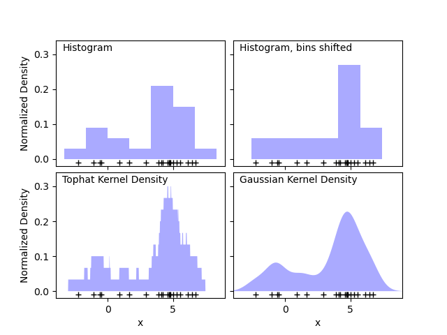
第一张图显示了使用直方图可视化一维点密度的问题之一。从直觉上讲，直方图可以看作是一种方案，其中将“块”单元堆叠在规则网格的每个点上方。但是，如前两个面板所示，这些块的网格选择可能导致有关密度分布的基本形状的想法大相径庭。如果我们改为将每个块放在其表示的点上居中，则得到的估计值将显示在左下方的面板中。这是使用“高顶礼帽”（top hat）核的内核密度估计。这个想法可以推广到其他核：第一个图的右下图显示了在相同分布上的高斯核密度估计。

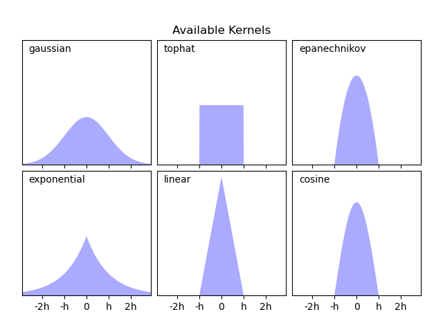
Scikit-learn通过sklearn.neighbors.KernelDensity估计器，使用Ball Tree或KD Tree结构实现了有效的内核密度估计。可用的核在本案例的第二张图中显示。

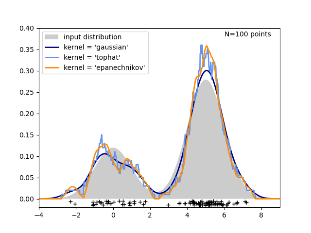
第三张图比较了在一维中分布100个样本的核密度估计。尽管此示例使用一维分布，但内核密度估计也可以轻松有效地扩展到更高的维度。

输入：

# 作者: Jake Vanderplas <jakevdp@cs.washington.edu>
#
import numpy as np
import matplotlib
import matplotlib.pyplot as plt
from distutils.version import LooseVersion
from scipy.stats import norm
from sklearn.neighbors import KernelDensity

# 在直方图中`normed`选项已经被弃用，现在更倾向于`density`
if LooseVersion(matplotlib.__version__) >= '2.1':
    density_param = {'density': True}
else:
    density_param = {'normed': True}

# ----------------------------------------------------------------------
# 绘制直方图到核的过程
np.random.seed(1)
N = 20
X = np.concatenate((np.random.normal(0, 1, int(0.3 * N)),
                    np.random.normal(5, 1, int(0.7 * N))))[:, np.newaxis]
X_plot = np.linspace(-5, 10, 1000)[:, np.newaxis]
bins = np.linspace(-5, 10, 10)

fig, ax = plt.subplots(2, 2, sharex=True, sharey=True)
fig.subplots_adjust(hspace=0.05, wspace=0.05)

# 直方图1
ax[0, 0].hist(X[:, 0], bins=bins, fc='#AAAAFF', **density_param)
ax[0, 0].text(-3.5, 0.31, "Histogram")

# 直方图2
ax[0, 1].hist(X[:, 0], bins=bins + 0.75, fc='#AAAAFF', **density_param)
ax[0, 1].text(-3.5, 0.31, "Histogram, bins shifted")

# 高礼帽核密度估计
kde = KernelDensity(kernel='tophat', bandwidth=0.75).fit(X)
log_dens = kde.score_samples(X_plot)
ax[1, 0].fill(X_plot[:, 0], np.exp(log_dens), fc='#AAAAFF')
ax[1, 0].text(-3.5, 0.31, "Tophat Kernel Density")

# 高斯核密度估计
kde = KernelDensity(kernel='gaussian', bandwidth=0.75).fit(X)
log_dens = kde.score_samples(X_plot)
ax[1, 1].fill(X_plot[:, 0], np.exp(log_dens), fc='#AAAAFF')
ax[1, 1].text(-3.5, 0.31, "Gaussian Kernel Density")

for axi in ax.ravel():
    axi.plot(X[:, 0], np.full(X.shape[0], -0.01), '+k')
    axi.set_xlim(-4, 9)
    axi.set_ylim(-0.02, 0.34)

for axi in ax[:, 0]:
    axi.set_ylabel('Normalized Density')

for axi in ax[1, :]:
    axi.set_xlabel('x')

# ----------------------------------------------------------------------
# 绘制所有可能的核函数
X_plot = np.linspace(-6, 6, 1000)[:, None]
X_src = np.zeros((1, 1))

fig, ax = plt.subplots(2, 3, sharex=True, sharey=True)
fig.subplots_adjust(left=0.05, right=0.95, hspace=0.05, wspace=0.05)


def format_func(x, loc):
    if x == 0:
        return '0'
    elif x == 1:
        return 'h'
    elif x == -1:
        return '-h'
    else:
        return '%ih' % x

for i, kernel in enumerate(['gaussian', 'tophat', 'epanechnikov',
                            'exponential', 'linear', 'cosine']):
    axi = ax.ravel()[i]
    log_dens = KernelDensity(kernel=kernel).fit(X_src).score_samples(X_plot)
    axi.fill(X_plot[:, 0], np.exp(log_dens), '-k', fc='#AAAAFF')
    axi.text(-2.6, 0.95, kernel)

    axi.xaxis.set_major_formatter(plt.FuncFormatter(format_func))
    axi.xaxis.set_major_locator(plt.MultipleLocator(1))
    axi.yaxis.set_major_locator(plt.NullLocator())

    axi.set_ylim(0, 1.05)
    axi.set_xlim(-2.9, 2.9)

ax[0, 1].set_title('Available Kernels')

# ----------------------------------------------------------------------
# 绘制一维密度评估的例子
N = 100
np.random.seed(1)
X = np.concatenate((np.random.normal(0, 1, int(0.3 * N)),
                    np.random.normal(5, 1, int(0.7 * N))))[:, np.newaxis]

X_plot = np.linspace(-5, 10, 1000)[:, np.newaxis]

true_dens = (0.3 * norm(0, 1).pdf(X_plot[:, 0])
             + 0.7 * norm(5, 1).pdf(X_plot[:, 0]))

fig, ax = plt.subplots()
ax.fill(X_plot[:, 0], true_dens, fc='black', alpha=0.2,
        label='input distribution')
colors = ['navy', 'cornflowerblue', 'darkorange']
kernels = ['gaussian', 'tophat', 'epanechnikov']
lw = 2

for color, kernel in zip(colors, kernels):
    kde = KernelDensity(kernel=kernel, bandwidth=0.5).fit(X)
    log_dens = kde.score_samples(X_plot)
    ax.plot(X_plot[:, 0], np.exp(log_dens), color=color, lw=lw,
            linestyle='-', label="kernel = '{0}'".format(kernel))

ax.text(6, 0.38, "N={0} points".format(N))

ax.legend(loc='upper left')
ax.plot(X[:, 0], -0.005 - 0.01 * np.random.random(X.shape[0]), '+k')

ax.set_xlim(-4, 9)
ax.set_ylim(-0.02, 0.4)
plt.show()

脚本的总运行时间：（0分钟0.620秒）